Application & Configuration¶

This section describes how to set up a new PopulationSim implementation.

In order to create a new PopulationSim implementation, the user must first understand the requirements of the project in terms of geographic resolution and details desired in the synthetic population. Once the requirements of the project have been established, the next step is to prepare the inputs to PopulationSim which includes seed population tables and geographic controls. Next, PopulationSim needs to be configured for available inputs and features desired in the final synthetic population. After this, the user needs to run PopulationSim and resolve any data related errors. Finally, the user should validate the output synthetic population against the controls to understand the precision of the synthetic population compared to controls and the amount of variance in the population for each control.

Selecting Geographies¶

PopulationSim can represent both household and person level controls at multiple geographic levels. Therefore the user must define what geographic units to use for each control. There is not necessarily any ‘right’ way to define geographic areas or to determine what geographic level to use for each control. However, there are important considerations for selecting geography, discussed below.

Traditionally, travel forecasting models have followed the sequential four-step model framework. This required the modeling region to be divided into zones, typically the size of census block groups or tracts. The zones used in four-step process are typically known as Transportation Analysis Zones (TAZs). The spatial boundaries of TAZs varies across modeling region and ranges from a city block to a large area in the suburb within a modeling region. If building a synthetic population for a trip-based model, or an activity-based travel models (ABMs) whose smallest geography is the TAZ, then there is no reason to select a smaller geoegraphical unit than the TAZ for any of the controls.

ABMs operate at the individual level, where travel decisions are modeled explicitly for persons and households in the synthetic population. Many ABMs operate at a finer spatial resolution than TAZs, wherein all location choices (e.g., usual work location, tour destination choice) are modeled at a sub-TAZ geography. This finer geography is typically referred to as Micro-Analysis Zones (MAZs) which are smaller zones nested within TAZs. Models that represent behavior at the MAZ level requires that MAZs are used as the lowest level of control, so that the synthetic population will identify the MAZ that each household resides in.

As discussed earlier, two main inputs to a population synthesizer are a seed sample and controls. The seed sample can come from a household travel survey or from American Community Survey (ACS) Public Use Microdata Sample (PUMS), with latter being the most common source. The PUMS data contains a sample of actual responses to the ACS, but the privacy of each household is protected by aggregating all household residential locations into relatively large regions called Public Use Microdata Areas (PUMAs). PUMAs are special non-overlapping areas that partition each state into contiguous geographic units containing no fewer than 100,000 people each. Some larger regions are composed of many PUMAs, while other, smaller regions have only one PUMA, or may even be smaller than a PUMA. It is not a problem to use PopulationSim to generate a synthetic population if the region is smaller than a PUMA; PopulationSim will ‘fit’ the PUMA-level population to regional control data as an initial step.

Often it is not possible or desirable to specify all the controls at the same level of geographic resolution. Some important demographic, socio-economic and land-use development distributions (e.g., employment or occupation data) which may be adopted for controls are only available at relatively aggregate geographies (e.g., County, District, Region, etc.). Moreover, some distributions which are available at a finer geographic level in the base year may not be available at the same geographic level for a future forecast year. In some cases, even if a control is available at a finer geography, the modeler might want to specify that control (e.g., population by age) at an aggregate geography due to concerns about accuracy, forecastability, etc.

The flexible number of geographies feature in PopulationSim enables user to make use of data available at different geographic resolutions. In summary, the choice of geographies for PopulationSim is decided based on following:

Travel Model Spatial Resolution: For most ABMs, this is MAZ but can also be TAZ or even Block Group
Availability of Control Data: Different controls are available at different geographic levels; some data is available at the block level (for example, total households), some data is avialable at the block group level, the tract level, the county level, etc.
Accuracy of Control Data: Generally there is more error in data specified at smaller geographic units than larger geographic units
Desired level of Control: It is possible that the user may not wish to control certain variables at a small geographic level, even if good base-year data were available. For example, the user may not have much faith in the ability to forecast certain variables at a small geogrphic level into the future. In such cases, the user may wish to aggregate available data to larger geographies.
Seed Sample Geography: The level at which seed data is specified automatically determines one of the geographic level (the Seed level).

The hierarchy of geographies is important when making a decision regarding controls. The hierarchy of geographies in PopulationSim framework is as follows:

Meta (e.g., the entire modeling region)

Seed (e.g., PUMA)

Sub-Seed (e.g., TAZ, MAZ)

The Meta geography is the entire region. PopulationSim can handle only one Meta geography. The Seed geography is the geographic resolution of the seed data. There can be one or more Seed geographies. PopulationSim can handle any number of nested Sub-Seed geographies. More information on PopulationSim algorithm can be found from the PopulationSim specifications in the Resources section.

Geographic Cross-walk¶

After selecting the geographies, the next step is to prepare a geographic cross-walk file. The geographic cross-walk file defines the hierarchical structure of geographies. The geographic cross-walk is used to aggregate controls specified at a lower geography to upper geography and to allocate population from an upper geography to a lower geography. An example geographic crosswalk is shown below:

TAZ	BLOCK GROUP	TRACT	PUMA	REGION
475	3	100	600	1
476	3	100	600	1
232	45	100	600	1
247	45	202	600	1
248	45	202	600	1

Preparing seed and control data¶

Seed sample¶

As mentioned in previous section, the seed sample is typically obtained from the ACS PUMS. One of the main requirements for the seed sample is that it should be representative of the modeling region. In the case of ACS PUMS, this can be ensured by selecting PUMAs representing the modeling region both demographically and geographically. PUMA boundaries may not perfectly line up against the modeling region boundaries and overlaps are possible. Each sub-seed geography must be assigned to a Seed geography, and each Seed geography must be assigned to a Meta geography.

The seed sample must contain all of the specified control variables, as well as any variables that are needed for the travel model but not specified as controls. For population groups that use completely separate, non-overlapping controls, such as residential population and group-quarter population, separate seed samples are prepared. In the ACS PUMS datasets, it is possible to have zero-person households in the raw data table (NP = 0); these records must be filtered from the seed data. PopulationSim can be set up and run separately for each population segment using the same geographic system. The outputs from each run can be combined into a unified synthetic population as a post processing step.

Finally, the seed sample must include an initial weight field. The PopulationSim algorithm is designed to assign weights as close to the initial weight as possible to minimize the changes in distribution of uncontrolled variables. All the fields in the seed sample should be appropriately recoded to specify controls (see more details in next section). Household-level population variables must be computed in advance (for e.g., number of workers in each household) and monetary variables must be inflation adjusted to be consistent with year of control data (e.g., Household Income). The ACS PUMS data contain 3 or 5 years of household records, where each record’s income is reported in the year in which it was collected. The ACS PUMS data includes the rolling reference factor for the year and the inflation adjustment factor, these must be used to code each household’s income to a common income year.

Controls¶

Controls are the marginal distributions that form the constraints for the population synthesis procedure. Controls are also referred to as targets and the objective of the population synthesis procedure is to produce a synthetic population whose attributes match these marginal distributions. Controls can be specified for both household and person variables. The choice of control variables depends on the needs of the project. Ideally, the user would want to specify control for all variables that are important determinant of travel behaviour or would be of interest to policy makers. These would include social, demographic, economic and land-use related variables.

The mandatory requirement for a population synthesizer is to generate the right number of households in each travel model geography. Therefore, it is mandatory to specify a control on total number of households in each geographical unit at the lowest geographical level. If this control is matched perfectly, it ensures that all the upper geographies also have the correct number of households assigned to them.

There are multiple source to obtain input data to build these controls. Most commonly, base-year controls are built from Census data, including Summary Files 1, 2 and 3, the American Community Survey, and the Census Transportation Planning Package (CTPP). Data from Census sources are typically available at one of the Census geographies - Census Block, Block Group, Census Tract, County, Metropolitan Statistical Area, etc. The modeling agency may collect important demographic data for the modeling region (e.g., number of households). Some data can also be obtained from a socio-economic or land-use model for the region such as, households by income groups or households by housing type.

Once the data has been obtained, it may be necessary to aggregate or disaggregate the data to the desired geography. Disaggregation involves distributing data from the upper geography to lower geographies using a distribution based on area, population or number of households. A simple aggregation is possible when the lower geography boundaries fits perfectly within the upper geography boundary. In case of overlaps, data can be aggregated in proportion to the area. A simpler method is to establish a correspondence between the lower and upper geography based on the position of the geometric centroid of the lower geography. If the centroid of the lower geography lies within the upper geography then the whole lower geography is assumed to lie within the upper geography. For some shapes, the geometric centroid might be outside the shape boundary. In such cases, an internal point closest to the geometric centroid but within the shape is used. All Census shape files come with the coordinates of the internal point. The user would need to download the Census shape files for the associated geography and then establish a correspondence with the desired geography using this methodology. It is recommended that input control data should be obtained at the lowest geography possible and then aggregated to the desired geography. These steps must be performed outside of PopulationSim, typically using a Geographic Information System (GIS) software program or travel modeling software package with GIS capabilities.

Control totals within a variable, such as households of size 1, 2, 3, and 4+, should be integerized and smart rounded if necessary since inconsistent controls make convergence more difficult. For example, if control data is allocated from Census geographies to TAZs, then often floating point controls are created. To correct this, one can calculate the difference between the floating point controls and integerized versions, and then add the error to the largest category by subtracting it from the other categories.

Configuration¶

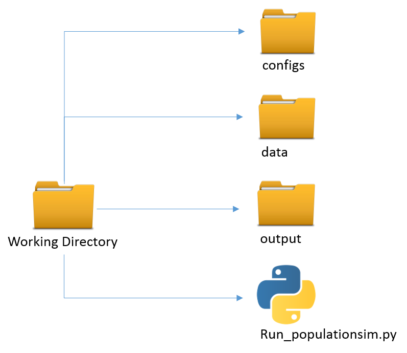
Below is PopulationSim’s typical directory structure followed by a description of inputs.

PopulationSim is run via run_populationsim.py. The user needs to first activate the popsim environment and then call the run_populationsim.py Python script to launch a PopulationSim run.

activate popsim
python run_populationsim.py

PopulationSim is configured using the settings.yaml file. PopulationSim can be configured to run in regular mode or repop mode.

regular mode: The regular configuration runs PopulationSim from beginning to end and produces a new synthetic population. This can run either single-process or multi-processed to save on runtime.
repop mode: The repop configuration is used for repopulating a subset of zones for an existing synthetic population. The user has the option to replace or append to the existing synthetic population. These options are specified from the settings.yaml file, details can be found in the Configuring Settings File section.

The following sections describes the inputs and outputs, followed by discussion on configuring the settings file and specifying controls.

Inputs & Outputs¶

Please refer to the following definition list to understand the file names:

GEOG_NAME: Sub-seed geography name such as TAZ, MAZ, etc.
SEED_GEOG: Geographic resolution of the seed sample such as PUMA.
META_GEOG: Geography name of the Meta geography such as Region, District, etc.

Working Directory Contents:

File	Description
run_populationsim.py	Python script that orchestrates a PopulationSim run
/configs	Sub-directory containing control specifications and configuration settings
/configs_mp	Sub-directory containing configuration settings for running multi-processed if applicable
/data	Sub-directory containing all input files
/output	Sub-directory containing all outputs, summaries and intermediate files

/configs Sub-directory Contents:

File	Description
logging.yaml	yaml-based file for setting up logging
settings.yaml	yaml-based settings file to configure a PopulationSim run
controls.csv	CSV file to specify controls

/configs_mp Sub-directory Contents:

File	Description
settings.yaml	additional yaml-based settings file for multiprocess running

/data Sub-directory Contents:

File	Description
control_totals_GEOG_NAME.csv	Marginal control totals at each spatial resolution named GEOG_NAME
geo_crosswalk.csv	Geographic cross-walk file
seed_households.csv	Seed sample of households
seed_persons.csv	Seed sample of persons

/output Sub-directory Contents (populated at the end of a PopulationSim run):

This sub-directory is populated at the end of the PopulationSim run. The table below list all possible outputs from a PopulationSim run. The user has the option to specify the output files that should be exported at the end of a run. Details can be found in the Configuring Settings File section.

File	Group	Description
asim.log	Logging	Log file
pipeline.h5	Data Pipeline	HDF5 data pipeline which stores all the inputs, outputs and intermediate files
expanded_household_ids.csv	Final Synthetic Population	List of expanded household IDs with their geographic assignment. User would join this file with the seed sample to generate a fully expanded synthetic population
synthetic_households.csv	Final Synthetic Population	Fully expanded synthetic population of households. User can specify the attributes to be included from the seed sample in the settings.yaml file
synthetic_persons.csv	Final Synthetic Population	Fully expanded synthetic population of persons. User can specify the attributes to be included from the seed sample in the settings.yaml file
incidence_table.csv	Intermediate	Intermediate incidence table
household_groups.csv	Intermediate	Unique household group assignments based on controls variables
GEOG_NAME_control_data.csv	Intermediate	Input control data at each geographic level - GEOG_NAME
GEOG_NAME_controls.csv	Intermediate	Control totals at each geographic level (GEOG_NAME) containing only the controls specified in the configs/controls.csv control specification file
GEOG_NAME_weights.csv	Intermediate	List of household weights with their geographic assignment
GEOG_NAME_weights_sparse.csv	Intermediate	List of household weights with their geographic assignment
control_spec.csv	Intermediate	Control specification used for the run
geo_cross_walk.csv	Intermediate	Input geographic cross-walk
crosswalk.csv	Intermediate	Trimmed geographic cross-walk used in PopulationSim run
trace_GEOG_NAME_weights.csv	Tracing	Trace file listing household weights for the trace geography specified in settings
summary_hh_weights.csv	Summary	List of household with weights through different stages of PopulationSim
summary_GEOG_NAME.csv	Summary	Marginal Controls vs. Synthetic Population Comparison at GEOG_NAME level
summary_GEOG_NAME_aggregate.csv	Summary	Household weights aggregate to SEED_GEOG at the end of allocation to GEOG_NAME
summary_GEOG_NAME_SEED_GEOG.csv	Summary	Marginal Controls vs. Synthetic Population Comparison at SEED_GEOG level using weights from allocation at GEOG_NAME level

Configuring Settings File¶

PopulationSim is configured using the configs/settings.yaml file. The user has the flexibility to specify algorithm functionality, list geographies, invoke tracing, provide inputs specifications, select outputs, list the steps to run, and specify multiprocess settings.

Note

When running PopulationSim, multiple settings files can be specified so long as the inherit_settings: True setting is included in subsequent files. This feature is used for the multi-processing configuration described below. To utilize this feature, once can run PopulationSim with the following command: python run_populationsim.py -c configs_mp -c configs. This command specifies two config folders, each with a settings file, and the configs_mp settings inherit from the earlier configs settings.

The settings shown below are from the PopulationSim application for the CALM region as an example of how a run can be configured. The meta geography for CALM region is named as Region, the seed geography is PUMA and the two sub-seed geographies are TRACT and TAZ. The settings below are for this four geography application, but the user can configure PopulationSim for any number of geographies and use different geography names.

Some of the setting are configured differently for the repop mode. The settings specific to the repop mode are described in the Configuring Settings File for repop Mode section. The settings specific to the multiprocessing setup are described in the Configuring Settings File for Multiprocessing section.

Algorithm/Software Configuration:

These settings control the functionality of the PopulationSim algorithm. The settings shown are currently the defaults as they were the ones used to validate the final PopulationSim application for the CALM region. They should not be changed by the casual user, with the possible exception of the max_expansion_factor setting, as explained below.

INTEGERIZE_WITH_BACKSTOPPED_CONTROLS: True
SUB_BALANCE_WITH_FLOAT_SEED_WEIGHTS: False
GROUP_BY_INCIDENCE_SIGNATURE: True
USE_SIMUL_INTEGERIZER: True
USE_CVXPY: False
max_expansion_factor: 30
MAX_BALANCE_ITERATIONS_SIMULTANEOUS: 1000

Attribute	Value	Description
INTEGERIZE_WITH_BACKSTOPPED_CONTROLS	True/False	When set to True, upper geography controls are imputed for current geography and used as additional controls for integerization
SUB_BALANCE_WITH_FLOAT_SEED_WEIGHTS	True/False	When True, PopulationSim uses floating weights from upper geography
GROUP_BY_INCIDENCE_SIGNATURE	True/False	When True, PopulationSim groups the household incidence by HH group
USE_SIMUL_INTEGERIZER	True/False	PopulationSim Integerizer can run in two modes: Sequential - Zones are processed in a ascending order of number of households in the zone Simultaneous - Zones are processed simultaneously for more details, refer the TRB paper on Docs page
USE_CVXPY	True/False	A third-party solver is used for integerization - CVXPY or or-tools CVXPY is currently not available for Windows
max_expansion_factor	> 0	Maximum HH expansion factor weight setting. This settings dictates the ratio of the final weight of the household record to its initial weight. For example, a maxExpansionFactor setting of 5 would mean a household having a PUMS weight of x can have a final weight of not more than 5x, thus effectively restricting the number of times a record can be sampled. The user might need to adjust this setting to enable sampling of a record with a rare household configuration. Otherwise, it might result in some controls not being matched due to unavailability of records to sample from. The maximum expansion factor may have to be adjusted upwards if the target is much greater than the seed number of households.
MAX_BALANCE_ITERATIONS_SIMULTANEOUS	Integer	Number of list balancer iterations. The default may be more than is needed.

Geographic Settings:

geographies: [REGION, PUMA, TRACT, TAZ]
seed_geography: PUMA

Attribute	Value	Description
geographies	List of geographies	List of geographies at which the controls are specified including the seed geography - PUMA. The geographies should be in the hierarchical order: REGION >> PUMA >> TRACT >> TAZ >> … Any number of geographies are allowed These geography names should be used as prefixes in control data file names for the corresponding geographies. Note that number of sub-seed geographies are flexible. Each must be listed in the run_list settings, shown below.
seed_geography	PUMA	Seed geography name from the list of geographies

Tracing:

Currently, only one unit can be listed. Only geographies below the seed geography can be traced.

trace_geography:
      TAZ: 100
      TRACT: 10200

Attribute	Description
TAZ	TAZ ID that should be traced.
TRACT	TRACT ID that should be traced.

data directory:

data_dir: data

Attribute	Description
data_dir	Name of the data_directory within the working directory. Do not change unless the directory structure changes from the template.

Input Data Tables

This setting is used to specify details of various inputs to PopulationSim. Below is the list of the inputs in the PopulationSim data pipeline:

Seed-Households

Seed-Persons

Geographic CrossWalk

Control data at each control geography

Note that Seed-Households, Seed-Persons and Geographic CrossWalk are all required tables and must be listed. There must be a control data file specified for each geography other than seed. For each input table, the user is required to specify an import table name, input CSV file name, index column name and column name map (only for renaming column names). The user can also specify a list of columns to be dropped from the input synthetic population seed data. An example is shown below followed by description of attributes.

input_table_list:
- tablename: households
        filename : seed_households.csv
        index_col: hh_id
        column_map:
        hhnum: hh_id
- tablename: persons
        filename : seed_persons.csv
        column_map:
        hhnum: hh_id
        SPORDER: per_num
        # drop mixed type fields that appear to have been incorrectly generated
        drop_columns:
        - indp02
        - naicsp02
        - occp02
        - socp00
        - occp10
        - socp10
        - indp07
        - naicsp07
- tablename: geo_cross_walk
        filename : geo_cross_walk.csv
        column_map:
        TRACTCE: TRACT
- tablename: TAZ_control_data
        filename : control_totals_taz.csv
- tablename: TRACT_control_data
        filename : control_totals_tract.csv
- tablename: REGION_control_data
        filename : scaled_control_totals_meta.csv

Attribute	Description
tablename	Name of the imported CSV file in the PopulationSim data pipeline. The input names in the PopulationSim data pipeline should be named as per the following standard: 1. Seed-Households - households Households across all Seed geographies should be in one file. There should be a Seed geography field with name as specified in the settings file. The seed geography identifies which Seed geography unit each household belongs to Seed-Persons - persons Persons across all Seed geographies should be in one file. There should be a Seed geography field with name as specified in the settings file. The seed geography identifies which Seed geography unit each person belongs to Geographic CrossWalk - geo_cross_walk The field names in the geographic cross-walk should be same as the geography names specified in the settings file Control data at each control geography - GEOG_NAME_control_data, where GEOG_NAME is the name of the control geography (TAZ, TRACT and REGION)
filename	Name of the input CSV file in the data folder
index_col	Name of the unique ID field in the seed household data
column_map	Column map of fields to be renamed. The format for the column map is as follows: `Name in CSV: New Name`
drop_columns	List of columns to be dropped from the input data

PopulationSim requires that the column names must be unqiue across all the control files. In case there are duplicate column names in the raw control files, user can use the column map feature to rename the columns appropriately.

Reserved Column Names:

Three columns representing the following needs to be specified:

Initial weight on households
Unique household identifier
Control on total number of households at the lowest geographic level

household_weight_col: WGTP
household_id_col: hh_id
total_hh_control: num_hh

Attribute	Description
household_weight_col	Initial weight column in the household seed sample
household_id_col	Unique household ID column in the household seed sample used to identify which persons are in which household. Should have same name as the index column on household seed table
total_hh_control	Total number of household control at the lowest geographic level. Note that PopulationSim requires this control to be specified at the lowest geography. It is strictly enforced

Control Specification File Name:

The control specification file is specified using a different token name for the repop mode as shown below.

control_file_name: controls.csv

Attribute	Description
control_file_name	Name of the CSV control specification file

Output Tables:

The output_tables: setting is used to control which outputs to write to disk. The Inputs & Outputs section listed all possible outputs. The user can specify either a list of output tables to include or to skip using the action attribute as shown below in the example. if neither is specified, then all output tables will be written. The HDF5 data pipeline and all summary files are written out regardless of this setting.

output_tables:
  action: include
  tables:
    - expanded_household_ids

Attribute	Description
action	include or skip the list of tables specified
tables	List of table to be written out or skipped

Synthetic Population Output Specification

This setting allows the user to specify the details of the expanded synthetic population. User can specify the output file names, household ID field name and the set of columns to be included from the seed sample.

output_synthetic_population:
  household_id: household_id
  households:
    filename: synthetic_households.csv
    columns:
      - NP
      - AGEHOH
      - HHINCADJ
      - NWESR
  persons:
    filename: synthetic_persons.csv
    columns:
      - per_num
      - AGEP
      - OSUTAG
      - OCCP

Attribute	Description
household_id	Column name of the unique household ID field in the expanded synthetic population
filename	CSV file names for the expanded households and persons table
columns	Names of seed sample columns to be included in the final synthetic population. Missing or misspelled column names generate error. The geographic allocation information of each household is added by default.

Steps for regular mode:

This setting lists the sub-modules or steps to be run by the PopulationSim orchestrator. The ActivitySim framework allows user to resume a PopulationSim run from a specific point. This is specified using the attribute resume_after. The step, sub_balancing.geography is repeated for each sub-seed geography (the example below shows two, but there can be 0 or more).

run_list:
  steps:
    - input_pre_processor
    - setup_data_structures
    - initial_seed_balancing
    - meta_control_factoring
    - final_seed_balancing
    - integerize_final_seed_weights
    - sub_balancing.geography=TRACT
    - sub_balancing.geography=TAZ
    - expand_households
    - write_results
    - summarize

  #resume_after: integerize_final_seed_weights

Attribute	Description
steps	List of steps to be run
resume_after	The step from which the current run should resume

For detailed information on software implementation refer to Core Components and Model Steps. The table below gives a brief description of each step.

Step	Description
input_pre_processor	Read input text files and save them as pipeline tables for use in subsequent steps.
setup_data_structures	Builds data structures such as incidence_table.
initial_seed_balancing	Balance the household weights for each of the seed geographies (independently) using the seed level controls and the aggregated sub-zone controls totals.
meta_control_factoring	Apply simple factoring to summed household fractional weights based on original meta control values relative to summed household fractional weights by meta zone.
final_seed_balancing	Balance the household weights for each of the seed geographies (independently) using the seed level controls and the aggregated sub-zone controls totals.
integerize_final_seed_weights	Final balancing for each seed (puma) zone with aggregated low and mid-level controls and distributed meta-level controls.
sub_balancing	Simul-balance and integerize all zones at a specified geographic level in groups by parent zone.
expand_households	Create a complete expanded synthetic household list with their assigned geographic zone ids.
write_tables	Write pipeline tables as csv files (in output directory) as specified by output_tables list in settings file.
write_synthetic_population	Write synthetic households and persons tables to output directory as csv files.
summarize	Write aggregate summary files of controls and weights for all geographic levels to output dir

Configuring Settings File for Multiprocessing¶

This sections describes the settings that are additionally configured for running PopulationSim with multiprocessing to reduce runtime. PopulationSim uses ActivitySim’s multiprocessing capabilities, which are described in more detail here.

The example below can be found in the example_calm\configs_mp\settings.yaml file. The group of model steps identified as mp_seed_balancing and starting with input_pre_processor are run single process until the next group of model steps identified as mp_sub_balancing_TAZ and starting with sub_balancing.geography=TAZ is reached, at which time PopulationSim runs these steps in parallel using two processors by slicing the problem into separate geographic batches based on the slice_geography: TRACT setting. It then returns to single process with the final group of model steps identified as mp_summarize and beginning with expand_households.

inherit_settings: True
multiprocess: True
num_processes: 2
cleanup_pipeline_after_run: True
slice_geography: TRACT

multiprocess_steps:
  - name: mp_seed_balancing
    begin: input_pre_processor
  - name: mp_sub_balancing_TAZ
    begin: sub_balancing.geography=TAZ
    num_processes: 2
    slice:
      tables:
        - slice_crosswalk
        - crosswalk
      # don't slice any tables not explicitly listed above in slice.tables
      except: True
      # the following tables are added by sub_balancer and should be coalesced
      coalesce:
        - TAZ_weights
        - TAZ_weights_sparse
        - trace_TAZ_weights
  - name: mp_summarize
    begin: expand_households

Attribute	Description
inherit_settings	True means this settings file inherits settings from settings file(s) identified earlier in the run command
num_processes	Number of processors to use for multiprocessing
cleanup_pipeline_after_run	Removes multiprocess process specific intermediate pipelines at the end of the run if desired
slice_geography	The geography used to separate the problem into parallel geographic batches for balancing
multiprocess_steps	Specifies which steps to run single process and multiprocess

Configuring Settings File for repop Mode¶

This sections describes the settings that are configured differently for the repop mode.

Input Data Tables for repop mode

The repop mode runs over an existing synthetic population and uses the data pipeline (HDF5 file) from the regular run as an input. User should copy the HDF5 file from the regular outputs to the output folder of the repop set up. The data input which needs to be specified in this setting is the control data for the subset of geographies to be modified. Input tables for the repop mode can be specified in the same manner as regular mode. However, only one geography can be controlled and the geography must be the lowest in “geographies” setting. In the example below, TAZ controls are specified. The controls specified in TAZ_control_data do not have to be consistent with the controls specified in the data used to control the initial population. Only those geographic units to be repopulated should be specified in the control data (for example, TAZs 314 through 317).

repop_input_table_list:
  - taz_control_data:
    filename : repop_control_totals_taz.csv
    tablename: TAZ_control_data

Control Specification File Name for repop mode:

repop_control_file_name: repop_controls.csv

Attribute	Description
repop_control_file_name	Name of the CSV control specification file for repop mode Must include total_hh_control field

Output Tables for repop mode:

It should be noted that only the summary_GEOG_NAME.csv summary file is available for the repop mode.

Steps for repop mode:

When running PoulationSim in repop mode, the steps specified in this setting are run. As mentioned earlier, the repop mode runs over an existing synthetic population. The default value for the resume_after setting under the repop mode is summarize which is the last step of a regular run. In other words, the repop mode starts from the last step of the regular run and modifies the regular synthetic population as per the new controls. The user can choose either append or replace in the expand_households.repop attribute to modify the existing synthetic population. The append option adds to the existing synthetic population in the specified geographies, while the replace option replaces any existing synthetic population with newly synthesized population in the specified geographies.

run_list:
  steps:
    - input_pre_processor.repop
    - repop_setup_data_structures
    - initial_seed_balancing.final=true
    - integerize_final_seed_weights.repop
    - repop_balancing
    # expand_households options are append or replace
    - expand_households.repop;replace
    - summarize.repop
    - write_synthetic_population.repop
    - write_tables.repop

  resume_after: summarize

Attribute	Description
steps	List of steps to be run Two options for the expand_households.repop step 1. append 2. replace
resume_after	The step from which the current run should resume

For information on software implementation of repop balancing refer to repop_balancing.

How to prepare PopulationSim inputs for survey weighting¶

The main difference in the seed sample for population synthesis and survey weighting is that in case of survey weighting the geographic allocation is known. PopulationSim operates at multiple geographies and performs geographic allocation of the sample to match controls at lower geographies. Since it is undesirable to change geographic allocation in case of survey weighting, controls should be specified only at one geographic level – the seed geography. All the other inputs must be prepared in the same fashion as for population synthesis.

Configuring PopulationSim for survey weighting:

Since survey weighting does not involve expanding the survey sample, integerization is not needed. Integerization can be skipped by switching off integerization in the yaml settings file as follows:

NO_INTEGERIZATION_EVER: True

User may want to specify the maximum and minimum limit on expansion of initial weights in the yaml settings file as follows:

max_expansion_factor: 4 # Default is 30
min_expansion_factor: 0.5

The desired output for survey weighting is a list of final weights by household ID. In order to achieve this, the grouping of incidence must be switched off in the yaml settings file as follows:

GROUP_BY_INCIDENCE_SIGNATURE: False

Output Tables for weighting mode:

To obtain the final weights by household ID, the seed geography weights table must be specified in the yaml settings file as below:

output_tables:
  action: include
  tables:
    - seed_geography_weights
    ...

The seed_geography_weights file contains the following columns:

HH_ID
SeedGeog_ID
preliminary_balanced_weight (weight after initial seed balancing)
sample_weight (initial sample weight)
balanced_weight (weight after final seed balancing)

Notes for weighting mode:

If there are no meta controls, the preliminary and final balanced weights are same.
It should be noted that under NO_INTEGERIZATION_EVER mode the expanded_household_ids file is empty.

Specifying Controls¶

The controls for a PopulationSim run are specified using the control specification CSV file. Following the ActivitySim framework, Python expressions are used for specifying control constraints. An example file is below.

target	geography	seed_table	importance	control_field	expression
num_hh	TAZ	households	100000000	HHBASE	(households.WGTP > 0) & (households.WGTP < np.inf) 1
hh_size_4_plus	TAZ	households	5000	HHSIZE4	households.NP >= 4
hh_age_15_24	TAZ	households	500	HHAGE1	(households.AGEHOH > 15) & (households.AGEHOH <= 24)
hh_inc_15	TAZ	households	500	HHINC1	(households.HHINCADJ > -999999999) & (households.HHINCADJ <= 21297)
student_fam_housing	TAZ	persons	500	OSUFAM	persons.OSUTAG == 1
hh_wrks_3_plus	TRACT	households	1000	HHWORK3	households.NWESR >= 3
hh_by_type_sf	TRACT	households	1000	SF	households.HTYPE == 1
persons_occ_8	REGION	persons	1000	OCCP8	persons.OCCP == 8

1: np.inf is the NumPy constant for infinty

Attribute definitions are as follows:

target: target is the name of the control in PopulationSim. A column by this name is added to the seed table. Note that the total_hh_control: target must be present in the control specification file. All other controls are flexible. The target names should be unique even if they are for different geographies.
geography: geography is the geographic level of the control, as specified in geographies.
seed_table: seed_table is the seed table the control applies to and it can be households or persons. If persons, then persons are aggregated to households using the count operator.
importance: importance is the importance weight for the control. A higher weight will cause PopulationSim to attempt to match the control at the possible expense of matching lower-weight controls. The importance weights are described in more detail in the What are importance weights and Setting importance weights sections.
control_field: control_field is the field in the control data input files that this control applies to. Note that the control field names should be unique even if they are for different geographies.
expression: expression is a valid Python/Pandas expression that identifies seed households or persons that this control applies to. The household and persons fields used for creating these expressions should exist in the seed tables. User might need to pre-process the seed sample to create the variable required in these expressions. These expressions can be specified for both discrete and continuous variables. For most applications, this involves creating logical relationships such as equalities, inequalities and ranges using the standard logical operators (AND, OR, EQUAL, Greater than, less than).

Some conventions for writing expressions:

Each expression is applied to all rows in the table being operated upon.
Expressions must be vectorized expressions and can use most numpy and pandas expressions.
When editing the CSV files in Excel, use single quote ‘ or space at the start of a cell to get Excel to accept the expression

What are importance weights¶

PopulationSim uses the relative entropy maximization-based list balancing to match controls specified at various geographic levels. The relative entropy-based optimization ensures that the least amount of new information is introduced in finding a feasible solution. The base entropy is defined by the initial weights in the seed sample. The weights generated by the entropy maximization algorithm preserve the distribution of initial weights while matching the marginal controls. This ensures that the resulting weights are both uniform and preserves the distribution of the uncontrolled variables in the seed sample. A general relative entropy optimization problem is formulated as:

\(\min\limits_{\rm x_{n}} \sum_{n}{x_{n}} ln\dfrac {x_{n}} {w_{n}}\)

Where \(x_{n}\) are the resulting household level weights, \(x_{n}\) are the initial weights. The marginal controls are specified as:

\(\sum_{n}{a_{in}*x_{n}} = A_{i}\)

In PopulationSim, the hard marginal controls are relaxed by use of slack or relaxation factors in the constraints as shown below:

\(\sum_{n}{a_{in}*x_{n}} = A_{i}*z_{i}\)

Where, \(z_{i}\) are relaxation factors and \(a_{in}\) are incidence values that map household/person attribute to marginal controls. To ensure that marginal controls are not relaxed significantly, the relaxation factors are also included in the objective function with a penalty. With control relaxations, the relative entropy optimization problem is formulated as follows:

\(\min\limits_{\rm x_{n}, z_{i}} \sum_{n}{x_{n}} ln\dfrac {x_{n}} {w_{n}} + \sum_{i}{u_{i}*(z_{i}ln{z_{i}})}\)

Where, \(u_{i}\) are the penalties termed as importance factors or importance weights in PopulationSim.

\(x_{n}\) and \(z_{i}\) are the parameters solved by the optimization while importance weights (\(u_{i}\)) are the hyperparameters that are exposed to the user and impact the optimization externally. The objective of the relative entropy optimization is to find a set of weights that are uniform and satisfy marginal controls. The importance weights allow the user to trade-off between these objectives. High importance weights (e.g., 1E10) on all controls result in a hard constrained optimization which gives a high preference to matching marginal controls. Low importance weights (e.g., <50) results in an almost unconstrained problem. The user may also specify different importance weights for each marginal control. In this case, the controls with higher importance weights are given preference over the ones with low importance weights. Therefore, both absolute and relative value of the importance weights impacts the optimization problem and the solution.

Setting importance weights¶

Given the flexibility that importance weights offer to the user, they need to be tuned to get the desired optimality in the outputs for the given seed sample and marginal controls. The quality of the outputs is defined by a uniformity measure of the weights and goodness of fit across marginal controls. Here are general guidelines on setting importance weights:

Start with a reasonable importance factor value across all controls (e.g., 1000 has typically worked well for multiple regions). This excludes the control on the total number of households which should be set to very high importance to ensure that the right number of households is generated for each zone.

After achieving reasonable goodness of fit across controls, the importance weights can be increased/decreased to favor one control over the other, or all importance weights can be reduced to improve the uniformity of the weights. Which controls to favor depends on the type of application and the quality of the marginal data.

The importance weights are generally updated in factors of 10. The user may need to run PopulationSim multiple times using various combinations of importance weights to reach the desired quality of outputs.

Error Handling & Debugging¶

It is recommended to do appropriate checks on input data before running PopulationSim. While the PopulationSim algorithm is designed to work even with imperfect data, an error-free and consistent set of input controls guarantees optimal performance. Poor performance and errors are usually the result of inconsistent data and it is the responsibility of the user to do necessary QA/QC on the input data. Some data problems that are frequently encountered are as follows:

Miscoding of data

Inconsistent controls (for example, household-level households by size controls do not match person-level controls on total persons, or household-level workers per household controls do not match person-level workers by occupation)

Controls do not add to total number of households

Controls do not aggregate consistently across geographies

Missing or mislabelled controls