Examples¶

This page describes the example models included with ActivitySim. The current examples are:

Example	Purpose	Zone Systems	Status
example_mtc	Primary MTC travel model one example	1	Mature
example_estimation	Estimation example with example_mtc	1	Mature
example_multiple_zones	2 or 3 zone system example using example_mtc data	2 or 3	Simple test example
example_marin	3 zone system example using Marin tour mode choice model	3	Mature
example_arc	ARC agency example	1	In development
example_semcog	SEMCOG agency example	1	In development
example_psrc	PSRC agency example	2	In development
example_sandag	SANDAG agency example	3	In development
example_sandag_xborder	SANDAG agency example	3	In development

Note

The example_manifest.yaml contains example commands to create and run several versions of the examples. See also Adding Agency Examples for more information on agency example models.

example_mtc¶

The initial example implemented in ActivitySim was example_mtc. This section described the example_mtc model design, how to setup and run the example, and how to review outputs. The default configuration of the example is limited to a small sample of households and zones so that it can be run quickly and require less than 1 GB of RAM. The full scale example can be configured and run as well.

Model Design¶

The example_mtc example is based on the Bay Area Metro Travel Model One (TM1). TM1 has its roots in a wide array of analytical approaches, including discrete choice forms (multinomial and nested logit models), activity duration models, time-use models, models of individual micro-simulation with constraints, entropy-maximization models, etc. These tools are combined in the model design to realistically represent travel behavior, adequately replicate observed activity-travel patterns, and ensure model sensitivity to infrastructure and policies. The model is implemented in a micro-simulation framework. Microsimulation methods capture aggregate outcomes through the representation of the behavior of individual decision-makers.

Space¶

TM1 uses the 1454 TAZ zone system developed for the MTC trip-based model. The zones are fairly large for the region, which may somewhat distort the representation of transit access in mode choice. To ameliorate this problem, the original model zones were further sub-divided into three categories of transit access: short walk, long walk, and not walkable. However, support for transit subzones is not included in the activitysim implementation since the latest generation of activity-based models typically use an improved approach to spatial representation called multiple zone systems. See example_multiple_zones for more information.

Decision-making units¶

Decision-makers in the model system are households and persons. These decision-makers are created for each simulation year based on a population synthesis process such as PopulationSim. The decision-makers are used in the subsequent discrete-choice models to select a single alternative from a list of available alternatives according to a probability distribution. The probability distribution is generated from various logit-form models which take into account the attributes of the decision-maker and the attributes of the various alternatives. The decision-making unit is an important element of model estimation and implementation, and is explicitly identified for each model.

Person type segmentation¶

TM1 is implemented in a micro-simulation framework. A key advantage of the micro-simulation approach is that there are essentially no computational constraints on the number of explanatory variables which can be included in a model specification. However, even with this flexibility, the model system includes some segmentation of decision-makers. Segmentation is a useful tool both to structure models and also as a way to characterize person roles within a household.

The person types shown below are used for the example model. The person types are mutually exclusive with respect to age, work status, and school status.

Person Type Code	Person Type	Age	Work Status	School Status
1	Full-time worker (30+ hours a week)	18+	Full-time	None
2	Part-time worker (<30 hours but works on a regular basis)	18+	Part-time	None
3	College student	18+	Any	College
4	Non-working adult	18 - 64	Unemployed	None
5	Retired person	65+	Unemployed	None
6	Driving age student	16 - 17	Any	Pre-college
7	Non-driving student	6 - 16	None	Pre-college
8	Pre-school child	0 - 5	None	Preschool

Household type segments are useful for pre-defining certain data items (such as destination choice size terms) so that these data items can be pre-calculated for each segment. Precalculation of these data items reduces model complexity and runtime. The segmentation is based on household income, and includes four segments - low, medium, high, very high.

In the model, the persons in each household are assigned a simulated but fixed value of time that modulates the relative weight the decision-maker places on time and cost. The probability distribution from which the value of time is sampled was derived from a toll choice model estimated using data from a stated preference survey performed for the SFCTA Mobility, Access, and Pricing Study, and is a lognormal distribution with a mean that varies by income segment.

Activity type segmentation¶

The activity types are used in most model system components, from developing daily activity patterns and to predicting tour and trip destinations and modes by purpose. The set of activity types is shown below. The activity types are also grouped according to whether the activity is mandatory or non-mandatory and eligibility requirements are assigned determining which person-types can be used for generating each activity type. The classification scheme of each activity type reflects the relative importance or natural hierarchy of the activity, where work and school activities are typically the most inflexible in terms of generation, scheduling and location, and discretionary activities are typically the most flexible on each of these dimensions. Each out-of-home location that a person travels to in the simulation is assigned one of these activity types.

Purpose	Description	Classification	Eligibility
Work	Working at regular workplace or work-related activities outside the home	Mandatory	Workers and students
University	College or university	Mandatory	Age 18+
High School	Grades 9-12	Mandatory	Age 14-17
Grade School	Grades preschool, K-8	Mandatory	Age 0-13
Escorting	Pick-up/drop-off passengers (auto trips only)	NonMandatory	Age 16+
Shopping	Shopping away from home	NonMandatory	Age 5+ (if joint travel, all persons)
Other Maintenance	Personal business/services and medical appointments	NonMandatory	Age 5+ (if joint travel, all persons)
Social/Recreational	Recreation, visiting friends/family	NonMandatory	Age 5+ (if joint travel, all persons)
Eat Out	Eating outside of home	NonMandatory	Age 5+ (if joint travel, all persons)
Other Discretionary	Volunteer work, religious activities	NonMandatory	Age 5+ (if joint travel, all persons)

Treatment of time¶

The TM1 example model system functions at a temporal resolution of one hour. These one hour increments begin with 3 AM and end with 3 AM the next day. Temporal integrity is ensured so that no activities are scheduled with conflicting time windows, with the exception of short activities/tours that are completed within a one hour increment. For example, a person may have a short tour that begins and ends within the 8 AM to 9 AM period, as well as a second longer tour that begins within this time period, but ends later in the day.

A critical aspect of the model system is the relationship between the temporal resolution used for scheduling activities and the temporal resolution of the network assignment periods. Although each activity generated by the model system is identified with a start time and end time in one hour increments, LOS matrices are only created for five aggregate time periods. The trips occurring in each time period reference the appropriate transport network depending on their trip mode and the mid-point trip time. The definition of time periods for LOS matrices is given below.

Time Period	Start Hour
EA	3
AM	5
MD	9
PM	14
EV	18

Trip modes¶

The trip modes defined in the example model are below. The modes include auto by occupancy and toll/non-toll choice, walk and bike, walk and drive access to five different transit line-haul modes, and ride hail with taxi, single TNC (Transportation Network Company), and shared TNC.

Auto

SOV Free

SOV Pay

2 Person Free

2 Person Pay

3+ Person Free

3+ Person Pay

Nonmotorized

Walk

Bike

Transit

Walk

Walk to Local Bus

Walk to Light-Rail Transit

Walk to Express Bus

Walk to Bus Rapid Transit

Walk to Heavy Rail

Drive

Drive to Local Bus

Drive to Light-Rail Transit

Drive to Express Bus

Drive to Bus Rapid Transit

Drive to Heavy Rail

Ride Hail

Taxi

Single TNC

Shared TNC

Sub-models¶

The general design of the example_mtc model is presented below. Long-term choices that relate to the usual workplace/university/school for each worker and student, household car ownership, and the availability of free parking at workplaces are first.

The coordinated daily activity pattern type of each household member is the first travel-related sub-model in the hierarchy. This model classifies daily patterns by three types:

Mandatory, which includes at least one out-of-home mandatory activity (work or school)

Non-mandatory, which includes at least one out-of-home non-mandatory activity, but does not include out-of-home mandatory activities

Home, which does not include any out-of-home activity or travel

The pattern type sub-model leaves open the frequency of tours for mandatory and nonmandatory purposes since these sub-models are applied later in the model sequence. Daily pattern-type choices of the household members are linked in such a way that decisions made by members are reflected in the decisions made by the other members.

After the frequency and time-of-day for work and school tours are determined, the next major model component relates to joint household travel. This component produces a number of joint tours by travel purpose for the entire household, travel party composition in terms of adults and children, and then defines the participation of each household member in each joint household tour. It is followed by choice of destination and time-ofday.

The next stage relates to maintenance and discretionary tours that are modeled at the individual person level. The models include tour frequency, choice of destination and time of day. Next, a set of sub-models relate tour-level details on mode, exact number of intermediate stops on each half-tour and stop location. It is followed by the last set of sub-models that add details for each trip including trip departure time, trip mode details and parking location for auto trips.

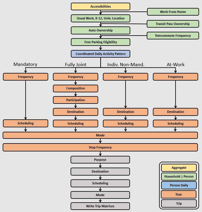
The output of the model is a disggregate table of trips with individual attributes for custom analysis. The trips can be aggregated into travel demand matrices for network loading.

Setup¶

The following describes the example_mtc model setup.

Folder and File Setup

The example_mtc has the following root folder/file setup:

configs - settings, expressions files, etc.

configs_mp - override settings for the multiprocess configuration

data - input data such as land use, synthetic population files, and network LOS / skims

output - outputs folder

Inputs¶

In order to run example_mtc, you first need the input files in the data folder as identified in the configs\settings.yaml file and the configs\network_los.yaml file:

input_table_list: the input CSV tables from MTC travel model one (see below for column definitions):
- households - Synthetic population household records for a subset of zones.
- persons - Synthetic population person records for a subset of zones.
- land_use - Zone-based land use data (population and employment for example) for a subset of zones.
taz_skims: skims.omx - an OMX matrix file containing the MTC TM1 skim matrices for a subset of zones. The time period for the matrix must be represented at the end of the matrix name and be seperated by a double_underscore (e.g. BUS_IVT__AM indicates base skim BUS_IVT with a time period of AM).

These files are used in the tests as well. The full set of MTC TM1 households, persons, and OMX skims are on the ActivitySim resources repository.

Additional details on these files is available in the original Travel Model 1 repository, although many of the files described there are not used in ActivitySim.

Households¶

The households table contains the following synthetic population columns:

household_id: numeric ID of this household, used in persons table to join with household characteristics
TAZ: zone where this household lives
income: Annual household income, in 2000 dollars
hhsize: Household size
HHT: Household type (see below)
auto_ownership: number of cars owned by this household (0-6)
num_workers: number of workers in the household
sample_rate

Household types¶

These are household types defined by the Census Bureau and used in ACS table B11001.

Code	Description
0	None
1	Married-couple family
2	Male householder, no spouse present
3	Female householder, no spouse present
4	Nonfamily household, male alone
5	Nonfamily household, male not alone
6	Nonfamily household, female alone
7	Nonfamily household, female not alone

Persons¶

This table describes attributes of the persons that constitute each household. This file contains the following columns:

person_id: Unique integer identifier for each person. This value is globally unique, i.e. no two individuals have the same person ID, even if they are in different households.
household_id: Household identifier for this person, foreign key to households table
age: Age in years
PNUM: Person number in household, starting from 1.
sex: Sex, 1 = Male, 2 = Female
pemploy: Employment status (see below)
pstudent: Student status (see below)
ptype: Person type (see person type segmentation above)

Employment status¶

Code	Description
1	Full-time worker
2	Part-time worker
3	Not in labor force
4	Student under 16

Student status¶

Code	Description
1	Preschool through Grade 12 student
2	University/professional school student
3	Not a student

Land use¶

All values are raw numbers and not proportions of the total.

TAZ: Zone which this row describes
DISTRICT: Superdistrict where this TAZ is (34 superdistricts in the Bay Area)
SD: Duplicate of DISTRICT
COUNTY: County within the Bay Area (see below)
TOTHH: Total households in TAZ
TOTPOP: Total population in TAZ
TOTACRE: Area of TAZ, acres
RESACRE: Residential area of TAZ, acres
CIACRE: Commercial/industrial area of TAZ, acres
TOTEMP: Total employment
AGE0519: Persons age 5 to 19 (inclusive)
RETEMPN: NAICS-based total retail employment
FPSEMPN: NAICS-based financial and professional services employment
HEREMPN: NAICS-based health, education, and recreational service employment
AGREMPN: NAICS-based agricultural and natural resources employment
MWTEMPN: NAICS-based manufacturing and wholesale trade employment
OTHEMP: NAICS-based other employment
PRKCST: Hourly cost paid by long-term (8+ hours) parkers, year 2000 cents
OPRKCST: Hourly cost paid by short term parkers, year 2000 cents
area_type: Area type designation (see below)
HSENROLL: High school students enrolled at schools in this TAZ
COLLFTE: College students enrolled full-time at colleges in this TAZ
COLLPTE: College students enrolled part-time at colleges in this TAZ
TERMINAL: Average time to travel from automobile storage location to origin/destination (floating-point minutes)

Counties¶

Code	Name
1	San Francisco
2	San Mateo
3	Santa Clara
4	Alameda
5	Contra Costa
6	Solano
7	Napa
8	Sonoma
9	Marin

Area types¶

Code	Description
0	Regional core
1	Central business district
2	Urban business
3	Urban
4	Suburban
5	Rural

Note

ActivitySim can optionally build an HDF5 file of the input CSV tables for use in subsequent runs since HDF5 is binary and therefore results in faster read times. see Configuration

OMX and HDF5 files can be viewed with the OMX Viewer or HDFView.

The other_resources\scripts\build_omx.py script will build one OMX file containing all the skims. The original MTC TM1 skims were converted from Cube to OMX using the other_resources\scripts\mtc_tm1_omx_export.s script.

The example_mtc inputs were created by the other_resources\scripts\create_sf_example.py script, which creates the land use, synthetic population, and skim inputs for a subset of user-defined zones.

Configuration¶

The configs folder contains settings, expressions files, and other files required for specifying model utilities and form. The first place to start in the configs folder is settings.yaml, which is the main settings file for the model run. This file includes:

models - list of model steps to run - auto ownership, tour frequency, etc. - see Pipeline
resume_after - to resume running the data pipeline after the last successful checkpoint
input_store - HDF5 inputs file
input_table_list - list of table names, indices, and column re-maps for each table in input_store
- tablename - name of the injected table
- filename - name of the CSV or HDF5 file to read (optional, defaults to input_store)
- index_col - table column to use for the index
- rename_columns - dictionary of column name mappings
- keep_columns - columns to keep once read in to memory to save on memory needs and file I/O
- h5_tablename - table name if reading from HDF5 and different from tablename
create_input_store - write new input_data.h5 file to outputs folder using CSVs from input_table_list to use for subsequent model runs
households_sample_size - number of households to sample and simulate; comment out to simulate all households
trace_hh_id - trace household id; comment out for no trace
trace_od - trace origin, destination pair in accessibility calculation; comment out for no trace
chunk_training_mode - disabled, training, production, or adaptive, see Chunk.
chunk_size - approximate amount of RAM in GBs to allocate to ActivitySim for batch processing choosers, see Chunk.
chunk_method - memory use measure such as hybrid_uss, see Chunk.
checkpoints - if True, checkpoints are written at each step; if False, no intermediate checkpoints will be written before the end of run; also supports an explicit list of models to checkpoint
check_for_variability - disable check for variability in an expression result debugging feature in order to speed-up runtime
log_alt_losers - if True, log (i.e. write out) expressions for debugging that return prohibitive utility values that exclude all alternatives. This feature slows down the model run and so it is recommended for debugging purposes only.
use_shadow_pricing - turn shadow_pricing on and off for work and school location
output_tables - list of output tables to write to CSV or HDF5
want_dest_choice_sample_tables - turn writing of sample_tables on and off for all models
cleanup_pipeline_after_run - if true, cleans up pipeline after successful run by creating a single-checkpoint pipeline file and deletes any subprocess pipelines
global variables that can be used in expressions tables and Python code such as:
- urban_threshold - urban threshold area type max value
- county_map - mapping of county codes to county names
- household_median_value_of_time - various household and person value-of-time model settings

Also in the configs folder is network_los.yaml, which includes network LOS / skims settings such as:

zone_system - 1 (taz), 2 (maz and taz), or 3 (maz, taz, tap)
taz_skims - skim matrices in one OMX file. The time period for the matrix must be represented at the end of the matrix name and be seperated by a double_underscore (e.g. BUS_IVT__AM indicates base skim BUS_IVT with a time period of AM.
skim_time_periods - time period upper bound values and labels
- time_window - total duration (in minutes) of the modeled time span (Default: 1440 minutes (24 hours))
- period_minutes - length of time (in minutes) each model time period represents. Must be whole factor of time_window. (Default: 60 minutes)
- periods - Breakpoints that define the aggregate periods for skims and assignment
- labels - Labels to define names for aggregate periods for skims and assignment
read_skim_cache - read cached skims (using numpy memmap) from output directory (memmap is faster than omx)
write_skim_cache - write memmapped cached skims to output directory after reading from omx, for use in subsequent runs
cache_dir - alternate dir to read/write cache files (defaults to output_dir)

Sub-Model Specification Files¶

Included in the configs folder are the model specification files that store the Python/pandas/numpy expressions, alternatives, and other settings used by each model. Some models includes an alternatives file since the alternatives are not easily described as columns in the expressions file. An example of this is the non_mandatory_tour_frequency_alternatives.csv file, which lists each alternative as a row and each columns indicates the number of non-mandatory tours by purpose. The set of files for the example_mtc are below. The example_arc example and example_semcog example added additional submodels.

Model	Specification Files
Initialize	initialize_landuse.yaml annotate_landuse.csv
Accessibility	accessibility.yaml accessibility.csv
Initialize	initialize_households.yaml annotate_persons.csv annotate_households.csv annotate_persons_after_hh.csv
School Location	school_location.yaml school_location_coeffs.csv annotate_persons_school.csv school_location_sample.csv tour_mode_choice.yaml (and related files) school_location.csv destination_choice_size_terms.csv shadow_pricing.yaml
School Location	workplace_location.yaml workplace_location_coeffs.csv annotate_persons_workplace.csv annotate_households_workplace.csv workplace_location_sample.csv tour_mode_choice.yaml (and related files) workplace_location.csv destination_choice_size_terms.csv shadow_pricing.yaml
Auto Ownership	auto_ownership.yaml auto_ownership_coeffs.csv auto_ownership.csv
Free Parking Eligibility	free_parking.yaml free_parking_coeffs.csv free_parking.csv free_parking_annotate_persons_preprocessor.csv
Coordinated Daily Activity Pattern	cdap.yaml annotate_persons_cdap.csv annotate_households_cdap.csv cdap_indiv_and_hhsize1.csv cdap_interaction_coefficients.csv cdap_fixed_relative_proportions.csv
Mandatory Tour Frequency	mandatory_tour_frequency.yaml mandatory_tour_frequency_coeffs.csv mandatory_tour_frequency.csv mandatory_tour_frequency_alternatives.csv annotate_persons_mtf.csv
Mandatory Tour Scheduling	mandatory_tour_scheduling.yaml tour_scheduling_work_coeffs.csv tour_scheduling_work.csv tour_scheduling_school.csv tour_departure_and_duration_alternatives.csv tour_departure_and_duration_segments.csv
Joint Tour Frequency	joint_tour_frequency.yaml joint_tour_frequency_coeffs.csv annotate_persons_jtf.csv joint_tour_frequency_annotate_households_preprocessor.csv joint_tour_frequency_alternatives.csv
Joint Tour Composition	joint_tour_composition.yaml joint_tour_composition_coefficients.csv joint_tour_composition_annotate_households_preprocessor.csv joint_tour_composition.csv
Joint Tour Participation	joint_tour_participation.yaml joint_tour_participation_coefficients.csv joint_tour_participation_annotate_participants_preprocessor.csv joint_tour_participation.csv
Joint Tour Destination Choice	joint_tour_destination.yaml non_mandatory_tour_destination_coefficients.csv non_mandatory_tour_destination_sample.csv non_mandatory_tour_destination.csv tour_mode_choice.yaml (and related files) destination_choice_size_terms.csv
Joint Tour Scheduling	joint_tour_scheduling.yaml tour_scheduling_joint_coefficients.csv joint_tour_scheduling_annotate_tours_preprocessor.csv tour_scheduling_joint.csv tour_departure_and_duration_alternatives.csv
Non-Mandatory Tour Frequency	non_mandatory_tour_frequency.yaml non_mandatory_tour_frequency_coefficients_{ptype}.csv non_mandatory_tour_frequency.csv non_mandatory_tour_frequency_alternatives.csv non_mandatory_tour_frequency_annotate_persons_preprocessor.csv non_mandatory_tour_frequency_extension_probs.csv annotate_persons_nmtf.csv
Non-Mandatory Tour Destination Choice	non_mandatory_tour_destination.yaml non_mandatory_tour_destination_coefficients.csv non_mandatory_tour_destination.csv non_mandatory_tour_destination_sample.csv tour_mode_choice.yaml (and related files) destination_choice_size_terms.csv
Non-Mandatory Tour Scheduling	non_mandatory_tour_scheduling.yaml tour_scheduling_nonmandatory_coefficients.csv non_mandatory_tour_scheduling_annotate_tours_preprocessor.csv tour_scheduling_nonmandatory.csv tour_departure_and_duration_alternatives.csv
Tour Mode Choice	tour_mode_choice.yaml tour_mode_choice_annotate_choosers_preprocessor.csv tour_mode_choice.csv tour_mode_choice_coefficients.csv tour_mode_choice_coeffs_template.csv
At-work Subtours Frequency	atwork_subtour_frequency.yaml atwork_subtour_frequency_coefficients.csv atwork_subtour_frequency.csv atwork_subtour_frequency_alternatives.csv atwork_subtour_frequency_annotate_tours_preprocessor.csv
At-work Subtours Destination Choice	atwork_subtour_destination.yaml atwork_subtour_destination_coefficients.csv atwork_subtour_destination_sample.csv atwork_subtour_destination.csv tour_mode_choice.yaml (and related files) destination_choice_size_terms.csv
At-work Subtour Scheduling	tour_scheduling_atwork.yaml tour_scheduling_atwork_coefficients.csv tour_scheduling_atwork.csv tour_scheduling_atwork_preprocessor.csv tour_departure_and_duration_alternatives.csv
At-work Subtour Mode	tour_mode_choice.yaml (and related files)
Intermediate Stop Frequency	stop_frequency.yaml stop_frequency_annotate_tours_preprocessor.csv stop_frequency_alternatives.csv stop_frequency_atwork.csv stop_frequency_eatout.csv stop_frequency_escort.csv stop_frequency_othdiscr.csv stop_frequency_othmaint.csv stop_frequency_school.csv stop_frequency_shopping.csv stop_frequency_social.csv stop_frequency_subtour.csv stop_frequency_univ.csv stop_frequency_work.csv
Trip Purpose	trip_purpose.yaml (+ trip_purpose_and_destination.yaml) trip_purpose_annotate_trips_preprocessor.csv trip_purpose_probs.csv
Trip Destination Choice	trip_destination.yaml (+ trip_purpose_and_destination.yaml) trip_destination.csv trip_destination_annotate_trips_preprocessor.csv trip_destination_sample.csv trip_mode_choice.yaml (and related files) destination_choice_size_terms.csv
Trip Scheduling (Probablistic)	trip_scheduling.yaml trip_scheduling_probs.csv
Trip Mode Choice	trip_mode_choice.yaml trip_mode_choice_annotate_trips_preprocessor.csv trip_mode_choice_coefficients.csv trip_mode_choice.csv
Parking Location Choice	parking_location_choice.yaml parking_location_choice_annotate_trips_preprocessor.csv parking_location_choice_coeffs.csv parking_location_choice.csv
Write Trip Matrices	write_trip_matrices.yaml write_trip_matrices_annotate_trips_preprocessor.csv

Pipeline¶

The models setting contains the specification of the data pipeline model steps, as shown below:

models:
   - initialize_landuse
   - compute_accessibility
   - initialize_households
   - school_location
   - workplace_location
   - auto_ownership_simulate
   - free_parking
   - cdap_simulate
   - mandatory_tour_frequency
   - mandatory_tour_scheduling
   - joint_tour_frequency
   - joint_tour_composition
   - joint_tour_participation
   - joint_tour_destination
   - joint_tour_scheduling
   - non_mandatory_tour_frequency
   - non_mandatory_tour_destination
   - non_mandatory_tour_scheduling
   - tour_mode_choice_simulate
   - atwork_subtour_frequency
   - atwork_subtour_destination
   - atwork_subtour_scheduling
   - atwork_subtour_mode_choice
   - stop_frequency
   - trip_purpose
   - trip_destination
   - trip_purpose_and_destination
   - trip_scheduling
   - trip_mode_choice
   - write_data_dictionary
   - track_skim_usage
   - write_trip_matrices
   - write_tables

These model steps must be registered Inject steps, as noted below. If you provide a resume_after argument to activitysim.core.pipeline.run() the pipeliner will load checkpointed tables from the checkpoint store and resume pipeline processing on the next model step after the specified checkpoint.

resume_after = None
#resume_after = 'school_location'

The model is run by calling the activitysim.core.pipeline.run() method.

pipeline.run(models=_MODELS, resume_after=resume_after)

Running the example¶

To run the example, do the following:

Activate the correct conda environment if needed
View the list of available examples

activitysim create --list

Create a local copy of an example folder

activitysim create --example example_mtc --destination my_test_example

Run the example

cd my_test_example
activitysim run -c configs -d data -o output

ActivitySim will log progress and write outputs to the output folder.

The example should run in a few minutes since it runs a small sample of households.

Note

A customizable run script for power users can be found in the Github repo. This script takes many of the same arguments as the activitysim run command, including paths to --config, --data, and --output directories. The script looks for these folders in the current working directory by default.

python simulation.py

Multiprocessing¶

The model system is parallelized via Multiprocessing. To setup and run the Examples using multiprocessing, follow the same steps as the above Running the example, but add an additional -c flag to include the multiprocessing configuration settings via settings file inheritance (see Command Line Interface) as well:

activitysim run -c configs_mp -c configs -d data -o output

The multiprocessing example also writes outputs to the output folder.

The default multiprocessed example is configured to run with two processors and chunking training: num_processes: 2, chunk_size: 0, and chunk_training_mode: training. Additional more performant configurations are included and commented out in the example settings file. For example, the 100 percent sample full scale multiprocessing example - example_mtc_full - was run on a Windows Server machine with 28 cores and 256GB RAM with the configuration below. The default setup runs with chunk_training_mode: training since no chunk cache file is present. To run the example significantly faster, try chunk_training_mode: disabled if the machine has sufficient RAM, or try chunk_training_mode: production. To configure chunk_training_mode: production, first configure chunking as discussed below. See Multiprocessing and Chunk for more information.

households_sample_size: 0
num_processes: 24
chunk_size: 0
chunk_training_mode: production

Configuring chunking¶

To configure chunking, ActivitySim must first be trained to determine reasonable chunking settings given the model setup and machine. The steps to configure chunking are:

Run the full scale model with chunk_training_mode: training. Set num_processors to about 80% of the available physical processors and chunk_size to about 80% of the available RAM. This will run the model and create the chunk_cache.csv file in the outputcache directory for reuse.
The households_sample_size for training chunking should be at least 1 / num_processors to provide sufficient data for training and the chunk_method: hybrid_uss typically performs best.
Run the full scale model with chunk_training_mode: production. Experiment with different num_processors and chunk_size settings depending on desired runtimes and machine resources.

See Chunk for more information. Users can run chunk_training_mode: disabled if the machine has an abundance of RAM for the model setup.

Outputs¶

The key output of ActivitySim is the HDF5 data pipeline file outputs\pipeline.h5. By default, this datastore file contains a copy of each data table after each model step in which the table was modified.

The example also writes the final tables to CSV files by using the write_tables step. This step calls activitysim.core.pipeline.get_table() to get a pandas DataFrame and write a CSV file for each table specified in output_tables in the settings.yaml file.

output_tables:
  h5_store: False
  action: include
  prefix: final_
  tables:
    - checkpoints
    - accessibility
    - land_use
    - households
    - persons
    - tours
    - trips
    - joint_tour_participants

The other_resources\scripts\make_pipeline_output.py script uses the information stored in the pipeline file to create the table below for a small sample of households. The table shows that for each table in the pipeline, the number of rows and/or columns changes as a result of the relevant model step. A checkpoints table is also stored in the pipeline, which contains the crosswalk between model steps and table states in order to reload tables for restarting the pipeline at any step.

Table	Creator	NRow	NCol
accessibility	compute_accessibility	1454	10
households	initialize	100	65
households	workplace_location	100	66
households	cdap_simulate	100	73
households	joint_tour_frequency	100	75
joint_tour_participants	joint_tour_participation	13	4
land_use	initialize_landuse	1454	44
person_windows	initialize_households	271	21
persons	initialize_households	271	42
persons	school_location	271	45
persons	workplace_location	271	52
persons	free_parking	271	53
persons	cdap_simulate	271	59
persons	mandatory_tour_frequency	271	64
persons	joint_tour_participation	271	65
persons	non_mandatory_tour_frequency	271	74
school_destination_size	initialize_households	1454	3
school_modeled_size	school_location	1454	3
tours	mandatory_tour_frequency	153	11
tours	mandatory_tour_scheduling	153	15
tours	joint_tour_composition	159	16
tours	tour_mode_choice_simulate	319	17
tours	atwork_subtour_frequency	344	19
tours	stop_frequency	344	21
trips	stop_frequency	859	7
trips	trip_purpose	859	8
trips	trip_destination	859	11
trips	trip_scheduling	859	11
trips	trip_mode_choice	859	12
workplace_destination_size	initialize_households	1454	4
workplace_modeled_size	workplace_location	1454	4

Logging¶

Included in the configs folder is the logging.yaml, which configures Python logging library. The following key log files are created with a model run:

activitysim.log - overall system log file
timing_log.csv - submodel step runtimes
omnibus_mem.csv - multiprocessed submodel memory usage

Refer to the Tracing section for more detail on tracing.

Trip Matrices¶

The write_trip_matrices step processes the trips table to create open matrix (OMX) trip matrices for assignment. The matrices are configured and coded according to the expressions in the model step trip annotation file. See Write Trip Matrices for more information.

Tracing¶

There are two types of tracing in ActivtiySim: household and origin-destination (OD) pair. If a household trace ID is specified, then ActivitySim will output a comprehensive set (i.e. hundreds) of trace files for all calculations for all household members:

Several CSV files - each input, intermediate, and output data table - chooser, expressions/utilities, probabilities, choices, etc. - for the trace household for each sub-model

If an OD pair trace is specified, then ActivitySim will output the acessibility calculations trace file:

accessibility.result.csv - accessibility expression results for the OD pair

With the set of output CSV files, the user can trace ActivitySim calculations in order to ensure they are correct and/or to help debug data and/or logic errors.

Writing Logsums¶

The tour and trip destination and mode choice models calculate logsums but do not persist them by default. Mode and destination choice logsums are essential for re-estimating these models and can therefore be saved to the pipeline if desired. To save the tour and trip destination and mode choice model logsums, include the following optional settings in the model settings file. The data is saved to the pipeline for later use.

# in workplace_location.yaml for example
DEST_CHOICE_LOGSUM_COLUMN_NAME: workplace_location_logsum
DEST_CHOICE_SAMPLE_TABLE_NAME: workplace_location_sample

# in tour_mode_choice.yaml for example
MODE_CHOICE_LOGSUM_COLUMN_NAME: mode_choice_logsum

The DEST_CHOICE_SAMPLE_TABLE_NAME contains the fields in the table below. Writing out the destination choice sample table, which includes the mode choice logsum for each sampled alternative destination, adds significant size to the pipeline. Therefore, this feature should only be activated when writing logsums for a small set of households for model estimation.

Field	Description
chooser_id	chooser id such as person or tour id
alt_dest	destination alternative id
prob	alternative probability
pick_count	sampling with replacement pick count
mode_choice_logsum	mode choice logsum

example_estimation¶

ActivitySim includes the ability to re-estimate submodels using choice model estimation tools such as larch. In order to do so, ActivitySim adopts the concept of an estimation data bundle (EDB), which is a collection of the necessary data to re-estimate a submodel. See Estimation for examples that illustrate running ActivitySim in estimation mode and using larch to re-restimate submodels.

example_multiple_zones¶

In a multiple zone system approach, households, land use, and trips are modeled at the microzone (MAZ) level. MAZs are smaller than traditional TAZs and therefore make for a more precise system. However, when considering network level-of-service (LOS) indicators (e.g. skims), the model uses different spatial resolutions for different travel modes in order to reduce the network modeling burden and model runtimes. The typical multiple zone system setup is a TAZ zone system for auto travel, a MAZ zone system for non-motorized travel, and optionally a transit access points (TAPs) zone system for transit.

ActivitySim supports models with multiple zone systems. The three versions of multiple zone systems are one-zone, two-zone, and three-zone.

One-zone: This version is based on TM1 and supports only TAZs. All origins and destinations are represented at the TAZ level, and all skims including auto, transit, and non-motorized times and costs are also represented at the TAZ level.

Two-zone: This version is similar to many DaySim models. It uses microzones (MAZs) for origins and destinations, and TAZs for specification of auto and transit times and costs. Impedance for walk or bike all-the-way from the origin to the destination can be specified at the MAZ level for close together origins and destinations, and at the TAZ level for further origins and destinations. Users can also override transit walk access and egress times with times specified in the MAZ file by transit mode. Careful pre-calculation of the assumed transit walk access and egress time by MAZ and transit mode is required depending on the network scenario.

Three-zone: This version is based on the SANDAG generation of CT-RAMP models. Origins and destinations are represented at the MAZ level. Impedance for walk or bike all-the-way from the origin to the destination can be specified at the MAZ level for close together origins and destinations, and at the TAZ level for further origins and destinations, just like the two-zone system. TAZs are used for auto times and costs. The difference between this system and the two-zone system is that transit times and costs are represented between Transit Access Points (TAPs), which are essentially dummy zones that represent transit stops or clusters of stops. Transit skims are built between TAPs, since there are typically too many MAZs to build skims between them. Often multiple sets of TAP to TAP skims (local bus only, all modes, etc.) are created and input to the demand model for consideration. Walk access and egress times are also calculated between the MAZ and the TAP, and total transit path utilities are assembled from their respective components - from MAZ to first boarding TAP, from first boarding to final alighting TAP, and from alighting TAP to destination MAZ. This assembling is done via the Transit Virtual Path Builder (TVPB), which considers all possible combinations of nearby boarding and alighting TAPs for each origin destination MAZ pair.

Regions that have an interest in more precise transit forecasts may wish to adopt the three-zone approach, while other regions may adopt the one or two-zone approach. The microzone version requires coding households and land use at the microzone level. Typically an all-streets network is used for representation of non-motorized impedances. This requires a routable all-streets network, with centroids and connectors for microzones. If the three-zone system is adopted, procedures need to be developed to code TAPs from transit stops and populate the all-street network with TAP centroids and centroid connectors. A model with transit virtual path building takes longer to run than a traditional TAZ only model, but it provides a much richer framework for transit modeling.

Note

The two and three zone system test examples are simple test examples developed from the TM1 example. To develop the two zone system example, TM1 TAZs were labeled MAZs, each MAZ was assigned a TAZ, and MAZ to MAZ impedance files were created from the TAZ to TAZ impedances. To develop the three zone example system example, the TM1 TAZ model was further transformed so select TAZs also became TAPs and TAP to TAP skims and MAZ to TAP impedances files were created. While sufficient for initial development, these examples were insufficient for validation and performance testing of the new software. As a result, the example_marin example was created.

Example simple test configurations and inputs for two and three-zone system models are described below.

Examples¶

To run the two zone and three zone system examples, do the following:

Activate the correct conda environment if needed
Create a local copy of the example

# simple two zone example
activitysim create -e example_2_zone -d test_example_2_zone

# simple three zone example
activitysim create -e example_3_zone -d test_example_3_zone

Change to the example directory
Run the example

# simple two zone example
activitysim run -c configs_2_zone -c configs -d data_2 -o output_2

# simple three zone example, single process and multiprocess (and makes use of settings file inheritance for running)
activitysim run -c configs_3_zone -c configs -d data_3 -o output_3 -s settings_static.yaml
activitysim run -c configs_3_zone -c configs -d data_3 -o output_3 -s settings_mp.yaml

Settings¶

Additional settings for running ActivitySim with two or three zone systems are specified in the settings.yaml and network_los.yaml files. The settings are:

Two Zone¶

In settings.yaml:

want_dest_choice_presampling - enable presampling for multizone systems, which means first select a TAZ using the sampling model and then select a microzone within the TAZ based on the microzone share of TAZ size term.

In network_los.yaml:

The additional two zone system settings and inputs are described and illustrated below. No additional utility expression files or expression revisions are required beyond the one zone approach. The MAZ data is available as zone data and the MAZ to MAZ data is available using the existing skim expressions. Users can specify mode utilities using MAZ data, MAZ to MAZ impedances, and TAZ to TAZ impedances.

zone_system - set to 2 for two zone system
maz - MAZ data file, with MAZ ID, TAZ, and land use and other MAZ attributes
maz_to_maz:tables - list of MAZ to MAZ impedance tables. These tables are read as pandas DataFrames and the columns are exposed to expressions.
maz_to_maz:max_blend_distance - in order to avoid cliff effects, the lookup of MAZ to MAZ impedance can be a blend of origin MAZ to destination MAZ impedance and origin TAZ to destination TAZ impedance up to a max distance. The blending formula is below. This requires specifying a distance TAZ skim and distance columns from the MAZ to MAZ files. The TAZ skim name and MAZ to MAZ column name need to be the same so the blending can happen on-the-fly or else a value of 0 is returned.

(MAZ to MAZ distance) * (distance / max distance) * (TAZ to TAZ distance) * (1 - (distance / max distance))

maz_to_maz:blend_distance_skim_name - Identify the distance skim for the blending calculation if different than the blend skim.

zone_system: 2
maz: maz.csv

maz_to_maz:
  tables:
    - maz_to_maz_walk.csv
    - maz_to_maz_bike.csv

  max_blend_distance:
    DIST: 5
    DISTBIKE: 0
    DISTWALK: 1

  blend_distance_skim_name: DIST

Three Zone¶

In addition to the extra two zone system settings and inputs above, the following additional settings and inputs are required for a three zone system model. Examples values are illustrated below.

In settings.yaml:

models - add initialize_los and initialize_tvpb to load network LOS inputs / skims and pre-compute TAP to TAP utilities for TVPB. See Initialize LOS.
want_dest_choice_presampling - enable presampling for multizone systems, which means first select a TAZ using the sampling model and then select a microzone within the TAZ based on the microzone share of TAZ size term.

models:
  - initialize_landuse
  - compute_accessibility
  - initialize_households
  # ---
  - initialize_los
  - initialize_tvpb
  # ---
  - school_location
  - workplace_location

In network_los.yaml:

zone_system - set to 3 for three zone system
rebuild_tvpb_cache - rebuild and overwrite existing pre-computed TAP to TAP utilities cache
trace_tvpb_cache_as_csv - write a CSV version of TVPB cache for tracing
tap_skims - TAP to TAP skims OMX file name. The time period for the matrix must be represented at the end of the matrix name and be seperated by a double_underscore (e.g. BUS_IVT__AM indicates base skim BUS_IVT with a time period of AM).
tap - TAPs table
tap_lines - table of transit line names served for each TAP. This file is used to trimmed the set of nearby TAP for each MAZ so only TAPs that are further away and serve new service are included in the TAP set for consideration. It is a very important file to include as it can considerably reduce runtimes.
maz_to_tap - list of MAZ to TAP access/egress impedance files by user defined mode. Examples include walk and drive. The file also includes MAZ to TAP impedances.
maz_to_tap:{walk}:max_dist - max distance from MAZ to TAP to consider TAP
maz_to_tap:{walk}:tap_line_distance_col - MAZ to TAP data field to use for TAP lines distance filter
demographic_segments - list of user defined demographic_segments for pre-computed TVPB impedances. Each chooser is coded with a user defined demographic segment.
TVPB_SETTINGS:units - specify the units for calculations, e.g. utility or time.
TVPB_SETTINGS:path_types - user defined set of TVPB path types to be calculated and available to the mode choice models. Examples include walk transit walk (WTW), drive transit walk (DTW), and walk transit drive (WTD).
TVPB_SETTINGS:path_types:{WTW}:access - access mode for the path type
TVPB_SETTINGS:path_types:{WTW}:egress - egress mode for the path type
TVPB_SETTINGS:path_types:{WTW}:max_paths_across_tap_sets - max paths to keep across all skim sets, for example, 3 TAP to TAP pairs per origin MAZ destination MAZ pair
TVPB_SETTINGS:path_types:{WTW}:max_paths_per_tap_set - max paths to keep per skim set, for example 1 per skim set - all transit submodes, local bus only, etc.

Unlike the one and two zone system approach, the three zone system approach requires additional expression files for the TVPB. The additional expression files for the TVPB are:

TVPB_SETTINGS:tap_tap_settings:SPEC - TAP to TAP expressions, e.g. tvpb_utility_tap_tap.csv
TVPB_SETTINGS:tap_tap_settings:PREPROCESSOR:SPEC - TAP to TAP chooser preprocessor, e.g. tvpb_utility_tap_tap_annotate_choosers_preprocessor.csv
TVPB_SETTINGS:maz_tap_settings:walk:SPEC - MAZ to TAP {walk} expressions, e.g. tvpb_utility_walk_maz_tap.csv
TVPB_SETTINGS:maz_tap_settings:drive:SPEC - MAZ to TAP {drive} expressions, e.g. tvpb_utility_drive_maz_tap.csv
TVPB_SETTINGS:accessibility:tap_tap_settings:SPEC - TAP to TAP expressions for the accessibility calculator, e.g. tvpb_accessibility_tap_tap.csv
TVPB_SETTINGS:accessibility:maz_tap_settings:walk:SPEC - MAz to TAP {walk} expressions for the accessibility calculator, e.g. tvpb_accessibility_walk_maz_tap.csv

Additional settings to configure the TVPB are:

TVPB_SETTINGS:tap_tap_settings:attribute_segments:demographic_segment - TVPB pre-computes TAP to TAP total utilities for demographic segments. These are defined using the attribute_segments keyword. In the example below, the segments are demographic_segment (household income bin), tod (time-of-day), and access_mode (drive, walk).
TVPB_SETTINGS:maz_tap_settings:{walk}:CHOOSER_COLUMNS - input impedance columns to expose for TVPB calculations.
TVPB_SETTINGS:maz_tap_settings:{walk}:CONSTANTS - constants for TVPB calculations.
accessibility:... - for the accessibility model step, the same basic set of TVPB configurations are available.

zone_system: 3

rebuild_tvpb_cache: False
trace_tvpb_cache_as_csv: False
tap_skims: tap_skims.omx
tap: tap.csv
maz_to_tap:
  walk:
    table: maz_to_tap_walk.csv
  drive:
    table: maz_to_tap_drive.csv

demographic_segments: &demographic_segments
- &low_income_segment_id 0
- &high_income_segment_id 1

TVPB_SETTINGS:
  tour_mode_choice:
    units: utility
    path_types:
      WTW:
        access: walk
        egress: walk
        max_paths_across_tap_sets: 3
        max_paths_per_tap_set: 1
      DTW:
        access: drive
        egress: walk
        max_paths_across_tap_sets: 3
        max_paths_per_tap_set: 1
      WTD:
        access: walk
        egress: drive
        max_paths_across_tap_sets: 3
        max_paths_per_tap_set: 1
    tap_tap_settings:
      SPEC: tvpb_utility_tap_tap.csv
      PREPROCESSOR:
        SPEC: tvpb_utility_tap_tap_annotate_choosers_preprocessor.csv
        DF: df
      attribute_segments:
        demographic_segment: *demographic_segments
        tod: *skim_time_period_labels
        access_mode: ['drive', 'walk']
      attributes_as_columns:
        - demographic_segment
        - tod
    maz_tap_settings:
      walk:
        SPEC: tvpb_utility_walk_maz_tap.csv
        CHOOSER_COLUMNS:
          - walk_time
      drive:
        SPEC: tvpb_utility_drive_maz_tap.csv
        CHOOSER_COLUMNS:
          - drive_time
          - DIST
    CONSTANTS:
      c_ivt_high_income: -0.028
      ...

  accessibility:
    units: time
    path_types:
      WTW:
        access: walk
        egress: walk
        max_paths_across_tap_sets: 1
        max_paths_per_tap_set: 1
    tap_tap_settings:
      SPEC: tvpb_accessibility_tap_tap_.csv
    maz_tap_settings:
        walk:
          SPEC: tvpb_accessibility_walk_maz_tap.csv
          CHOOSER_COLUMNS:
            - walk_time
    CONSTANTS:
        out_of_vehicle_walk_time_weight: 1.5
        out_of_vehicle_wait_time_weight: 2.0

Outputs¶

Essentially the same set of outputs is created for a two or three zone system model as for a one zone system model. However, the one key additional bit of information for a three zone system model is the boarding TAP, alighting TAP, and transit skim set is added to the relevant chooser table (e.g. tours and trips) when the chosen mode is transit. Logging and tracing also work for two and three zone models, including tracing of the TVPB calculations. The Write Trip Matrices step writes both TAZ and TAP level matrices depending on the configured number of zone systems.

Presampling¶

In multiple zone systems models, destination choice presampling is activated by default. Destination choice presampling first aggregates microzone size terms to the TAZ level and then runs destination choice sampling at the TAZ level using the destination choice sampling models. After sampling X number of TAZs based on impedance and size, the model selects a microzone for each TAZ based on the microzone share of TAZ size. Presampling significantly reduces runtime while producing similar results.

example_marin¶

To finalize development and verification of the multiple zone system and transit virtual path building components, the Transportation Authority of Marin County version of MTC travel model two (TM2) work tour mode choice model was implemented. This example was also developed to test multiprocessed runtime performance. The complete runnable setup is available from the ActivitySim command line interface as example_3_marin_full. This example has essentially the same configuration as the simpler three zone example above.

Example¶

To run example_marin, do the following:

Activate the correct conda environment if needed
Create a local copy of the example

# Marin TM2 work tour mode choice for the MTC region
activitysim create -e example_3_marin_full -d test_example_3_marin_full

Change to the example directory
Run the example

# Marin TM2 work tour mode choice for the MTC region
activitysim run -c configs -d data -o output -s settings_mp.yaml

For optimal performance, configure multiprocessing and chunk_size based on machine hardware.

Settings¶

Additional settings for running the Marin TM2 tour mode choice example are in the network_los.yaml file. The only additional notable setting is the tap_lines setting, which identifies a table of transit line names served for each TAP. This file is used to trimmed the set of nearby TAP for each MAZ so only TAPs that are further away and serve new service are included in the TAP set for consideration. It is a very important file to include as it can considerably reduce runtimes.

tap_lines: tap_lines.csv

example_arc¶

Note

This example is in development

The example_arc added a Trip Scheduling Choice (Logit Choice), Trip Departure Choice (Logit Choice), and Parking Location Choice submodel. These submodel specification files are below, and are in addition to the example_mtc submodel Sub-Model Specification Files.

Example ARC Sub-Model Specification Files¶

Model	Specification Files
Trip Scheduling Choice (Logit Choice)	trip_scheduling_choice.yaml trip_scheduling_choice_preprocessor.csv trip_scheduling_choice.csv
Trip Departure Choice (Logit Choice)	trip_departure_choice.yaml trip_departure_choice_preprocessor.csv trip_departure_choice.csv
Parking Location Choice	parking_location_choice.yaml parking_location_choice_annotate_trips_preprocessor.csv parking_location_choice_coeffs.csv parking_location_choice.csv

Example¶

See example commands in example_manifest.yaml for running example_arc. For optimal performance, configure multiprocessing and chunk_size based on machine hardware.

example_semcog¶

Note

This example is in development

The example_semcog added a Work From Home, Telecommute Frequency, Transit Pass Subsidy and Transit Pass Ownership submodel. These submodel specification files are below, and are in addition to the example_mtc submodel Sub-Model Specification Files. These submodels were added to example_semcog as extensions, which is a way for users to add submodels within their model setup as opposed to formally adding them to the activitysim package. Extension submodels are run through the models settings. However, the model must be run with the simulation.py script instead of the command line interface in order to load the extensions folder.

Example SEMCOG Sub-Model Specification Files¶

Model	Specification Files
Work From Home	work_from_home.yaml work_from_home.csv work_from_home_coeffs.csv
Telecommute Frequency	telecommute_frequency.yaml telecommute_frequency.csv telecommute_frequency_coeffs.csv
Transit Pass Subsidy	transit_pass_subsidy.yaml transit_pass_subsidy.csv transit_pass_subsidy_coeffs.csv
Transit Pass Ownership	transit_pass_ownership.yaml transit_pass_ownership.csv transit_pass_ownership_coeffs.csv

Example¶

See example commands in example_manifest.yaml for running example_semcog. For optimal performance, configure multiprocessing and chunk_size based on machine hardware.

example_psrc¶

Note

This example is in development

The example_psrc is a two zone system (MAZs and TAZs) implementation of the example_mtc model design. It uses PSRC zones, land use, synthetic population, and network LOS (skims).

Example¶

See example commands in example_manifest.yaml for running example_psrc. For optimal performance, configure multiprocessing and chunk_size based on machine hardware.

example_sandag¶

Note

This example is in development

The example_sandag is a three zone system (MAZs, TAZs, and TAPs) implementation of the example_mtc model design. It uses SANDAG zones, land use, synthetic population, and network LOS (skims).

Example¶

See example commands in example_manifest.yaml for running example_sandag. For optimal performance, configure multiprocessing and chunk_size based on machine hardware.

example_sandag_xborder¶

Note

This example is in development

The example_sandag_xborder is a three zone system (MAZs, TAZs, and TAPs) that generates cross-border activities for a tour-based population of Mexican residents. In addition to the normal SANDAG zones, there are external MAZs and TAZs defined for each border crossing station (Port of Entry). Because the model is tour-based, there are no household or person-level attributes in the synthetic population. The principal difference between this and the standard 3-zone implementation is that since household do not have a default tour origin (home zones), a tour OD choice model is required to assign tour origins and destinations simultaneously.

Example¶

See example commands in example_manifest.yaml for running example_sandag_xborder. For optimal performance, configure multiprocessing and chunk_size based on machine hardware.